If you have ever tried to rank columns of data based on variables present in other columns, you probably have realised that there is no easy way to do so, either in Microsoft Excel or Google Sheets.
After hitting this obstacle a while back, I eventually found how you could do the equivalent of a =RANKIF formula in Google Sheets. This is going to be a short article so let’s get right into it.
The Dataset
This is the dataset we are going to focus on ranking depending on different parameters.
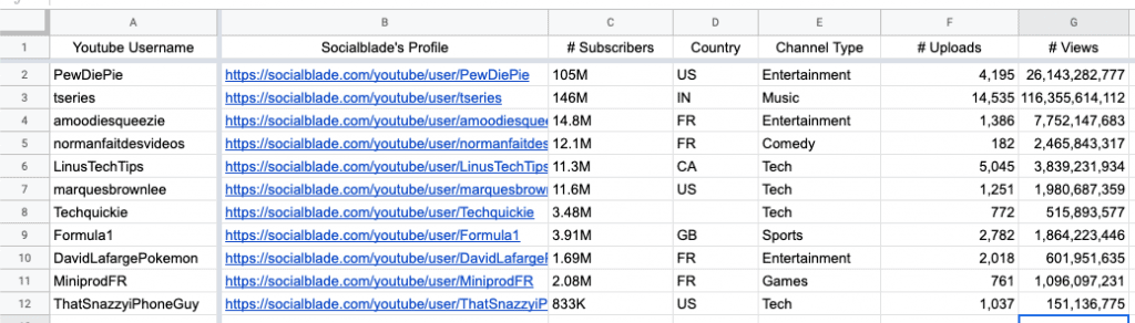
This is a list of Youtube Channels with information that is updated in real-time (If you are interested in building your own Youtube Channels Monitoring Dashboard in Google Sheets, you can read my tutorial here). As you can see, some of these columns like “Country” or “Channel Type” are easy prospects for our test here.
Our goal here is to rank these channels by how many views they have had and by their countries of origin. Basically, I want to see which Youtube channel has had the most views in the US, in France and in every country I might add to this dataset later.
RANKIF based on another column’s data in Google Sheets
The first thing we want to look at is how the RANK formula works.
The first argument this formula takes is the value to rank. The second argument is which dataset the first value should be compared to.
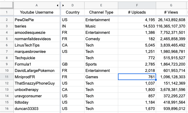
If we would want to rank the channels based on the overall amount of views they had, this is what we would do:
But this is not what we want. We want it ranked based on the column “Country”, that is the column D.
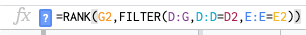
In order to do that, we are going to apply a FILTER formula to the second variable of the RANK formula. This is how it looks:
The FILTER formula basically removes every row out of the equation of the RANK formula that is not the equivalent of the country where the Youtube channel is from.
In this case, a literal translation of the formula in H2 would be:
Rank the value 26M+ (G2) out of every other value in the column G if they have US (D2) in column D (D:D=D2).
As you may notice in the FILTER formula requirements, you can have multiple conditions simultaneously if you want to use the RANK function depending on more factors.
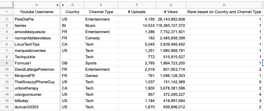
Now, let’s say we would want to rank every Youtube channel based on its Country of origin AND the Channel Type (Entertainment, tech, etc.)
As you can see, we now have a bunch of channels originating from the US and in the Tech space:
Now, we simply need to add a new condition to our FILTER formula like so:
And this is it, now the RANK formula only ranks youtube channels based on their views that share the same country of origin and the same channel type variable.
Conclusion
As you can see, this was a short article compared but I believe this can reveal itself useful for many people. As usual, if you encounter any issue while trying to replicate this endeavour, feel free tor each out to me by email or through the comments section down below and I will try to get back to you as soon as I can.
Thank you for your time,


3 Responses
Is it possible to use this formula and give a weight to each colomn?
For example:
=RANK(T14,FILTER(Q:U,Q:Q=Q14,R:R=R14,S:S=S14))
Q14 weights 40%
R14 weights 30%
S14 weights 30%
Please let me know, thanks!
This is great, Yaniss! Is there a way to wrap this in an arrayformula?
One issue with this approach is that, if you have two columns with the same types of data in them, that are both in the range, then the ranking will be across both columns.
For example, if, instead of Uploads, column F was another large number similar to Views, such as Subscribers, then those numbers would be included in the ranking.
Took me a few minutes to figure out that’s what was happening with my data. Fortunately, with only needing one filter column, it was easy enough to insert columns and copy paste the content across to the relevant location and then hide that column (for neatness).