Recently, I was asked how to remove all special characters from a cell in Google Sheets. This article is going to be short so here we go.
Using RegexReplace in Google Sheets
For the purpose of this article, we are going to use the formula =REGEXREPLACE. This is how it works:
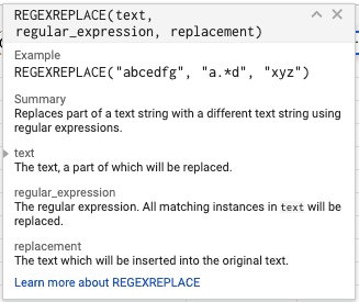
This formula allows us to replace text found in a cell using RE2. RE2 is short for Regular Expressions 2 and is a variant of the classic Regular Expressions by Google. If you are familiar with regex, you need to know that Google does not support every way you can use regex.
If you’re not familiar with Regular Expressions, you can read the Syntax Documentation that Google has made available on their Github repository at this address. For the purpose of this article, I will just share the answer and not go into details on what you can do with RE2 but you are free to study this document and do your own experimentations.
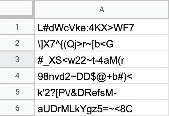
Our dataset today consists of a list of strong passwords that I created using the Password generator at passwordgenerator.net . There is no purpose to this tutorial other than experimenting with RE2 and having fun.
Here is the dataset:
Replacing Characters with REGEXREPLACE
Now that we have our dataset, here is how we are going to write our formula:

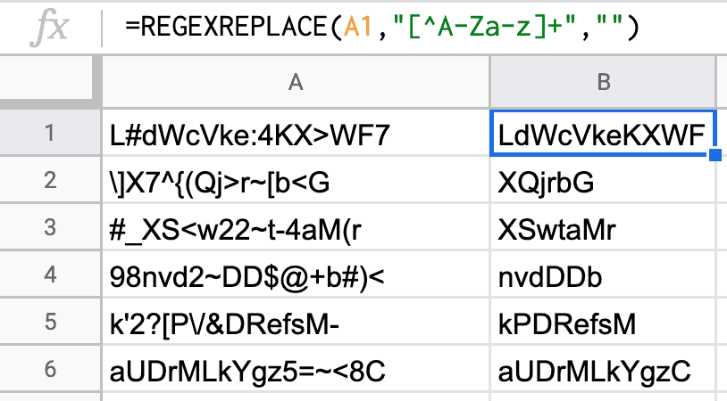
=REGEXREPLACE(A1,"[^A-Za-z]+","")In common words, this is what it means: In the Cell A1, find every character that is not between a-z and A-Z and replace it with nothing.
The ^ sign basically means opposite of. In this case, opposite of alphabet characters. The + after the brackets means that this formula applies for the whole string and not just for the first time a character matches this formula
And this is the result if we drag down this formula in front of the dataset I showed earlier:
Conclusion
And this is it really. I know this is a short article but it really was just for the benefit of experimentation. I hope this formula is going to reveal itself useful for some of you. If you have any questions, don’t hesitate to leave me a comment in the section below.
Thank you for your time. Until the next one !