Update from the 15th of April 2021: It appears that the source that was feeding this spreadsheet tutorial has drastically changed the way their interface was operating, rendering this whole tutorial pretty much useless. I am looking for a new source of data but at this moment, the easy way I was showing in this article is unfortunately not working anymore. I am truly sorry for that and as I said, I will be working towards making this tutorial great again 😎
This article is the last one of a series that is looking into creating your own Social Media Monitoring spreadsheets to spy on your competitors or monitor the health of your clients’ accounts. This specific article is about retrieving the data of Instagram Accounts and automatically putting them in Google Sheets.
We are still going to use the website SocialBlade for the same reasons as before: Code simplicity.
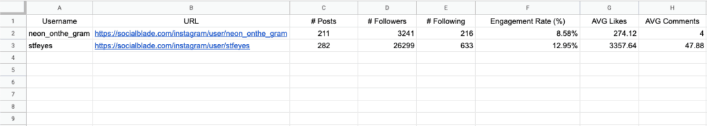
In this tutorial, I want to focus my effort on being able to display the followers/following count, the number of posts made, the engagement rate of the account and the average number of likes and comments for each account. Ready? Let’s do that.
PS: If you’re not interested in learning how to do your own spreadsheet (No judgment), there’s a protected spreadsheet that you can make a copy of at the end of this article so feel free to use it.
Using =IMPORTXML To Extract Web-Page Content
Once again, the formula “IMPORTXML” is going to be the driver of this project. IMPORTXML is basically a web-scraper built-in Google Sheets.
This is how it works:
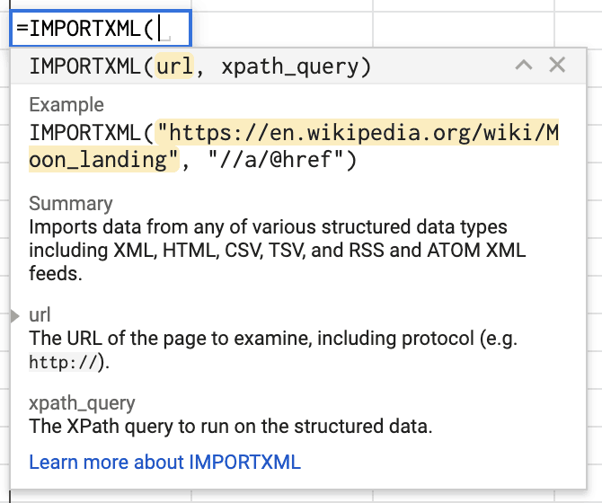
The way this function works is by taking two parameters: The URL where the data is stored and the exact emplacement inside the URL where the data is located in XPath format.
I will work you through how XPath works for our case but here’s a link to the documentation found on W3Schools if you are interested: https://www.w3schools.com/xml/xpath_syntax.asp
Now let’s take a look at one of my Instagram accounts (@neon_onthe_gram) on Socialblade (Link: https://socialblade.com/instagram/user/neon_onthe_gram)

As stated previously, these are the informations we’re going to extract from the webpage to put in our Google Spreadsheet.
If you “Inspect” (Right-Click -> Inspect) the number “211” that is the number of followers I have, you will get access to these information:

If you have a bit of HTML knowledge, you can figure out that every <div> that has the class “YouTubeuserTopInfo” contains one of the segments of the data we’re trying to extract. Unfortunately, the actual value we are interested in is not stored in an HTML tag that is easy to identify (Note: The number “211” is stored in a <span> tag that does not have any “id” or “class” attribute.). In practicality, it just means that we are going to have to extract the six “div” in their entirety and then split the data to remove the text and only keep the numbers.
The good news is, because the six divs we’re interested in all share the same class, it makes it really easy for us to get this data in a table format like so:
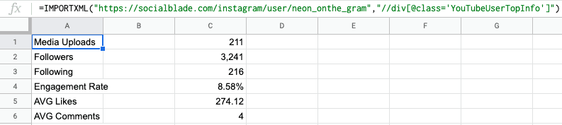
This single formula generated all of the cells displayed in the image above.
Now, the tricky part is to just keep the last column of this data (The column C with the values) and put it in a line instead of a column to be able to sort the values easily once we are going to display.
To do so, we’re going to use a combination of the formula TRANSPOSE and INDEX. Here’s the formula:
The purpose of the INDEX function is to specify that out of the table output generated by the IMPORTXML function, we only want to display every row of the third column.
The TRANSPOSE function is a simple function that inverts the direction of a range of cells so instead of having the output displayed vertically, we can have it displayed horizontally.
Creating the Dynamic Spreadsheet
Now that we have the formula that extracts the data we are looking for, we just have to dynamically create the URLs where the data is stored for every username we are interested in.
The first step to get this going is to get the columns ready like so:

The goal here is to type in the username of an account in
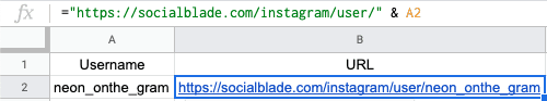
You can copy paste the block below:
="https://socialblade.com/instagram/user/" & A2This will ensure that by dragging down the cell B2, the URL that will be displayed will always reflect the one of the username in front of it.
Now we need to create the IMPORTXML function so it uses the Cell reference in the B column and can also be dragged down to automatically reflect the URL in front of itself.
And the code here:
=TRANSPOSE(INDEX(IMPORTXML(B2,"//div[@class='YouTubeUserTopInfo']"),0,3))Now you can drag down both B2 and C2:
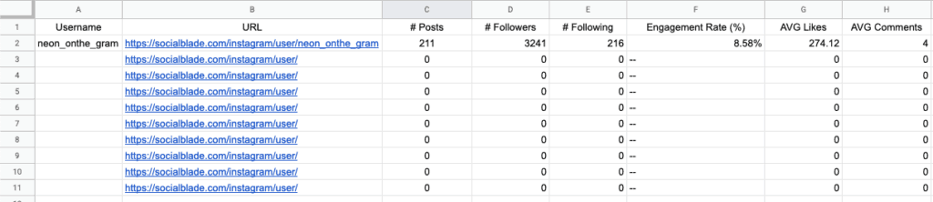
As you can notice, this is not the cleanest looking sheet with all of those #REF errors. The secret here is to add a formula in front of the formula present in B2 and C2:
=if(A2="","","https://socialblade.com/instagram/user/" & A2)One way to read this one is “If Username cell is empty, show nothing. Otherwise, create the URL based on Username”
And we can do the same with the C column:
=if(A2="","",TRANSPOSE(INDEX(IMPORTXML(B2,"//div[@class='YouTubeUserTopInfo']"),0,3)))Now, that’s how our spreadsheet look like if we drag down the cells B2 and C2:
Link to the Spreadsheet
Although I just explained how to do the whole spreadsheet yourself, I understand you might just want to use it. If oyu’re just interested in the spreadsheet, here is the link to the file you can make a copy of for your own Google Drive for your own usage: https://docs.google.com/spreadsheets/d/1mVaCROebN-UXnLwzt5olBA0x6kIFSJuOnrptvyj0Wto/edit?usp=sharing
Conclusion
And that’s pretty much it. I hope you will have find this subject interesting.
If you have any question, feel free to leave a reply down below or shoot me an email and I will get back to you as soon as I can.
Also consider subscribing to my Marketing Technology Newsletter if this topic interested you. I’m in no shortage of articles ideas around this subject and am also sharing new tools I’m experimenting with as well as articles from other insightful websites to help you stay up-to-date with the latest trends in the field.
See you next time!


24 Responses
Just looking through your sheet, it’s awesome! Do you know a way to automatically update the results daily?
Hey, thanks for reaching out! So actually the updating of the spreadsheet can not be controlled whatsoever in my experience. However, I found when I created this post that on a 50-70 rows spreadsheets with 4 columns, all of the values would get updated every 36-48 hours if I at least opened the spreadsheet once a day. By looking into it it looks like Google is monitoring how often a sheet is looked at to trigger the IMPORTXML update.
Tbh I’m going to look into it more in-depth. I’ll add that to my to-do list as I see that no one really figured how often and what can trigger an IMPORTXML update so that could be a nice article as well 😀 Will keep you updated of my discoveries!
Yaniss lot of thanks this is great. Question: AVG comments and likes are expressed per post? because you said per account but I don’t get that
Hey thank you so much for your comment! And yes my bad, AVG Comments and Likes are expressed per post :). Thank you for pointing it out, I’ll edit it!
Hi, I don’t know why but I have some problems.
I added usernames but instead of numbers I see “Loading…” and it loads forever…. 🙁
Hi, I’m having an issue here, when I import the xml instead of importing 6 lines, it imports a seventh line which says “help us by authenticating” and there’s no value to it, but when I transpose everything and keep only the values, this 7 line which now is a column, is empty, but whenever I type any value or word in this cell it erases all of the other values.
I’m not sure if I’m making myself clear, but what I want to know is how to import only the 6 lines that I want, and not this “help us by authenticating” line too.
Thanks
Hey, if we’re tracking instagram followers why does the code include YouTubeUserTopInfo?
Hi Tianna! Thank you for reaching out.
I was also confused at first but I believe it is just the way SocialBlade is built. They started their business by tracking Youtube channels and probably did not bother updating the name of the code structure when they also started offering other social media networks on their platform. But as long as you feed the formula an Instagram SocialBlade URL, the “YoutubeUserTopInfo” contains the data for the Instagram account 🙂
Hi!
Thanks for this – do you know what is happening, I am copying the formulas from your sheet into mine and they work, when I change them to one of my pages: @iriszajac they still work, but not for @raw.vegan.cakes
Any ideas?
Thanks so much for your help,
Iris
Been using this amazing monitoring sheets for the past 5 months! It’s amazing how you came up with this. Thank you so much! However, just about today I noticed that the engagement rate column stopped reflecting the numbers. Do you have any idea why that is?
Hi Stella! Wow, 5 months? I’m so happy to hear that aha, glad it has been useful :D! Thank you for the kind words 🙂
So I looked it up and it looks like SocialBlade changed their code a little bit, Rest assured, I found a way to restore the Engagement Rate data 🙂
You can find the updated code in this spreadsheet: https://docs.google.com/spreadsheets/d/1mVaCROebN-UXnLwzt5olBA0x6kIFSJuOnrptvyj0Wto/edit?usp=sharing
Hope this will work for you too 🙂 Thanks again for your comment, I really appreciate it!
Hi stella, can you give me this sheet? Thank you so much
Thank you so much for taking the time to put this together!! Do you know how to use your sheets if you have a large amount of data (8-9k rows) to track?
Hi Yanis,
great series of articles, thanks a lot !
It would appears you made a mistake in this sentence :
“The TRANSPOSE function is a simple function that inverts the direction of a range of cells so instead of having the output displayed vertically, we can have it displayed vertically.”
I think you wanted to say :
“The TRANSPOSE function is a simple function that inverts the direction of a range of cells so instead of having the output displayed vertically, we can have it displayed HORIZONTALLY”
Hi Tuhadj! Great catch, thank you very much for letting me know, I will update this sentence right away 🙂
And also thank you for the kind words, I really appreciate it 😀
Have you done this for Twitter? I tried changing “instagram” to “twitter” in the formula and using the twitter tag instead and it does pull numbers, but different numbers. Would love to see.
Hi Kendra!
Thank you for the comment. Actually yes, I have done this for Twitter as well but haven’t gotten around to make an article about it. but the spreadsheet already exists. it’s available at this link: https://docs.google.com/spreadsheets/d/1mVaCROebN-UXnLwzt5olBA0x6kIFSJuOnrptvyj0Wto/edit?usp=sharing . You will find it under the tab “Twitter” so you can just make a copy of the spreadsheet so you can start using it right away :).
Best,
Yaniss
Hi) Tell me please how to make the information imported vertically
Hi, it doesn’t work anymore somehow, even in your own spreadsheet – guess they have changed it again?
Ouch! It seems like they are hiding the data now… Hopefully they don’t do that for the other social medias… I will have to look at alternatives for Instagram in the meantime…
Thanks for pointing it out and I’m sorry you were not able to enjoy this spreadsheet before 🙁
Thanks for the heads up! Was really enjoying it and looking forward to your updates!
Hello
Its really helpfull… but now this formula was unable to use anymore, please update teh formula. since the result is N/A . Maybe it’s due to socialblade need to login to check Instagram ER.
Wating for your update and really appreciate it
Thank you